Data-To-Code Execution

Converting SQL text to an executable plan is termed Query Compilation, the subject of this page.

Figure 1. Query Compilation

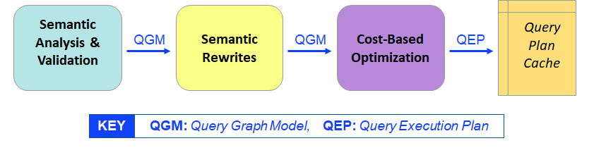
The SQL query is converted to a Query Execution Plan (QEP), a hierarchical structure that defines the steps to execute the query. The output from SQL EXPLAIN is a human-readable view of the QEP and, like the QEP, should be read from bottom to top.

Example Explain Plans

These examples use the data from our ice-hockey sample database - see NUODB_HOME/samples/quickstart/sql.

EXAMPLE 1: Find the first 10 players and list their names and approximate AGE value (to keep the diagram simple).

EXPLAIN
  SELECT firstname, lastname, YEAR(NOW()) - birthyear AS AGE
    FROM Players LIMIT 10;
 Rewritten Sub-expressions: [YEAR(NOW()) -> ?:1]
Project PLAYERS.FIRSTNAME, PLAYERS.LASTNAME, AGE
  Evaluation (?:1 - PLAYERS.BIRTHYEAR)
    Table scan PLAYERS limit 10 (cost: 1519.3, est. rows: 10)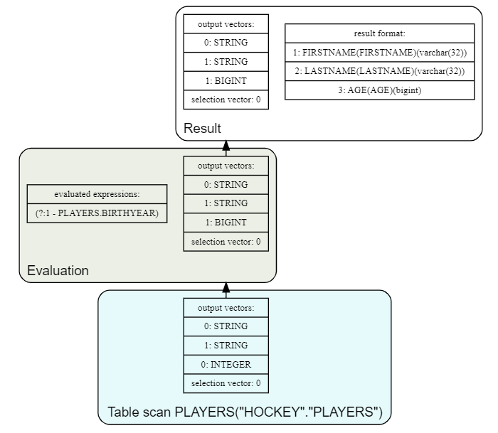

Figure 2. First explain plan visualized.

Reading in reverse order:

Scan the table finding the first 10 rows (no suitable index so a simple table-scan, row by row, is being used).
- Note the cost is small because it is not scanning all the rows, just 10 of them.
Evaluate the AGE for each row found.
Create the result set (projection).

Much easier to see in the diagram.

Note the rewriting rule: optimizes the evaluation by converting the function calls YEAR(NOW()) to a constant bind-variable ?:1.

EXAMPLE 2: Find the tallest ever 10 players, showing their height in feet and inches.

SQL> EXPLAIN
       SELECT firstname, lastname, height/12 AS FEET, height%12 AS INCHES
         FROM Players ORDER BY height DESC LIMIT 10;
 Project PLAYERS.FIRSTNAME, PLAYERS.LASTNAME, FEET, INCHES
  Evaluation (PLAYERS.HEIGHT / 12) (PLAYERS.HEIGHT % 12)
    Sort PLAYERS.HEIGHT DESC limit 10 (cost: 1335428.4, est. rows: 7520)
      Table scan PLAYERS (cost: 1141765.6, est. rows: 7520)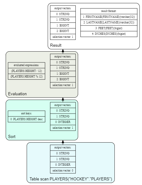

Figure 3. Second explain plan visualized.

Reading in reverse order:

Again scan the table to find rows.
- This time, all rows are needed so the cost is much higher.
Sort into descending order of height and choose just the first ten.
Calculate the FEET and INCHES columns.
Create the result set (projection).

Again the diagram shows the steps nicely.

Operators

The SQL query is broken down into a series of executable steps called Operators. A predefined set of operators are available for use and every query can be broken down into one or more operations. You will see these operators when reading explain plans so you must understand what they do.

Often there is a choice of possible operators and it is the job of the Optimizer to pick the best one. Internally NuoDB keeps statistics about each table and its indexes (such as the number of rows, how evenly the keys are distributed across the table) and generates cost estimates for each possible operator. Then it can choose the fastest. The most obvious example is the cost of a full table scan versus using a suitable index.

The Optimizer currently supports the following operators.

TableScan - process a table row by row.
BatchScan - fetches the rows indicated by a bitmap - see below.
NestedLoopsJoin - process a join between two tables.
Filter - filter predicates.
Projection - generates the final result set.
Sort - implements ORDER BY.
StreamedGrouping - implements GROUP BY.

Dedicated operators for processing indexes fall into two types.

Bitmap

Generates a bitmap, one bit per row in the table, where the bit is true if the row contains the key and false otherwise. This is best when only a small number of keys are likely to match the query (according to the cost-based analysis). Combining predicates can then be implemented quickly as AND or OR between the bitmaps.

Operators are: BitmapSource, BitmapUnion, BitmapIntersection.

Streaming

When many rows are likely to match the query, matching rows can be processed as a stream rather than processing all the rows upfront as the bitmap operator does. This reduces memory usage significantly for big tables. Rows are streamed in key order by scanning over the index.

Operators are: StreamingBatchScan, StreamingCoveringScan.

Working with Explain Plans

In an explain plan, to follow the steps of the query, start at the bottom of the plan and work up. Each step provides data for the step above it. Sometimes multiple steps provide data to the step above (For example, a join between two or more tables).

The optimizer does not always generate the best query, especially when you know more about the "shape" of the data than the cost analysis can determine. You can add query hints to the query to force it to use or ignore certain operators (most commonly indexes).

For more information, see Understanding EXPLAIN Command Output and Examples of Debugging a Slow Query.